Analyzing Image Classification Dataset

In this tutorial we use fastdup to analyze a labelled image classification dataset for potential issues.

By the end of this tutorial you'll learn how to:

• Load and format annotations in fastdup.
• Compare labels of similar images.
• Visualize a subset of the dataset using its labels.

Setting Up

You can follow along this tutorial by running this notebook on Google Colab.

First, install fastdup with:

bash

pip install fastdup

And verify the installation.

Python

import fastdup
fastdup.__version__

This tutorial runs on version 0.906.

Download Dataset

We will be analyzing the Imagenette dataset - A 10-class ImageNet subset from fast.ai.

Imagenette consists of 10 classes from the original ImageNet dataset. It contains 13k images in total.

Download and extract dataset:

shell

!wget https://s3.amazonaws.com/fast-ai-imageclas/imagenette2-160.tgz  
!tar -xzf imagenette2-160.tgz

Once done you should have a folder with the following structure.

./imagenette2-160/
├── noisy_imagenette.csv
├── train
│   ├── n01440764 
│   ├── n02102040 
│   ├── n02979186 
│   ├── n03000684 
│   ├── n03028079 
│   ├── n03394916 
│   ├── n03417042 
│   ├── n03425413 
│   ├── n03445777 
│   └── n03888257 
└── val
    ├── n01440764 
    ├── n02102040 
    ├── n02979186 
    ├── n03000684 
    ├── n03028079 
    ├── n03394916 
    ├── n03417042 
    ├── n03425413
    ├── n03445777 
    └── n03888257 

📘

Naming

• noisy_imagenette.csv - A .csv files with labels.
• train/ - Train images.
• val/ - validation images.

Load & Format Annotations

We'll use pandas to load and format the annotations.

Python

import pandas as pd

data_dir = 'imagenette2-160/'
csv_path = 'imagenette2-160/noisy_imagenette.csv'

As ImageNet uses codes for classes, we'll map them to their human readable values for ease of analysis (source):

Python

label_map = {
    'n02979186': 'cassette_player', 
    'n03417042': 'garbage_truck', 
    'n01440764': 'tench', 
    'n02102040': 'English_springer', 
    'n03028079': 'church',
    'n03888257': 'parachute', 
    'n03394916': 'French_horn', 
    'n03000684': 'chain_saw', 
    'n03445777': 'golf_ball', 
    'n03425413': 'gas_pump'
}

Let's load the annotations.

Python

df_annot = pd.read_csv(csv_path)
df_annot.head(3)

	path	noisy_labels_0	noisy_labels_1	noisy_labels_5	noisy_labels_25	noisy_labels_50	is_valid
0	train/n02979186/n02979186_9036.JPEG	n02979186	n02979186	n02979186	n02979186	n02979186	False
1	train/n02979186/n02979186_11957.JPEG	n02979186	n02979186	n02979186	n02979186	n03000684	False
2	train/n02979186/n02979186_9715.JPEG	n02979186	n02979186	n02979186	n03417042	n03000684	False

Transform the annotation into a format expected by fastdup.

Python

# take relevant columns
df_annot = df_annot[['path', 'noisy_labels_0']]

# rename columns to fastdup's column names
df_annot = df_annot.rename({'noisy_labels_0': 'label', 'path': 'img_filename'}, axis='columns')

# create split column
df_annot['split'] = df_annot['img_filename'].apply(lambda x: x.split("/")[0])

# map label ids to regular labels
df_annot['label'] = df_annot['label'].map(label_map)

# show formated annotations
df_annot.head()

	img_filename	label	split
0	train/n02979186/n02979186_9036.JPEG	cassette_player	train
1	train/n02979186/n02979186_11957.JPEG	cassette_player	train
2	train/n02979186/n02979186_9715.JPEG	cassette_player	train
3	train/n02979186/n02979186_21736.JPEG	cassette_player	train
4	train/n02979186/ILSVRC2012_val_00046953.JPEG	cassette_player	train

Run fastdup

With the annotations and folders in the right format, let's run fastdup and analyze the dataset.

Python

import fastdup
work_dir = 'fastdup_imagenette'

fd = fastdup.create(work_dir=work_dir, input_dir=data_dir) 
fd.run(annotations=df_annot, ccthreshold=0.9, threshold=0.8)

📘

Info

• ccthreshold - Threshold to use for the graph connected component. Default is 0.96.
• threshold - Threshold to use for the graph generation. Default is 0.9.

Get a summary of the run.

Python

fd.summary()

Dataset Analysis Summary: 

    Dataset contains 13394 images
    Valid images are 100.00% (13,394) of the data, invalid are 0.00% (0) of the data
    Similarity:  2.73% (366) belong to 20 similarity clusters (components).
    97.27% (13,028) images do not belong to any similarity cluster.
    Largest cluster has 40 (0.30%) images.
    For a detailed analysis, use `.connected_components()`
(similarity threshold used is 0.8, connected component threshold used is 0.9).

    Outliers: 6.20% (830) of images are possible outliers, and fall in the bottom 5.00% of similarity values.
    For a detailed list of outliers, use `.outliers()`.
['Dataset contains 13394 images',
 'Valid images are 100.00% (13,394) of the data, invalid are 0.00% (0) of the data',
 'Similarity:  2.73% (366) belong to 20 similarity clusters (components).',
 '97.27% (13,028) images do not belong to any similarity cluster.',
 'Largest cluster has 40 (0.30%) images.',
 'For a detailed analysis, use `.connected_components()`\n(similarity threshold used is 0.8, connected component threshold used is 0.9).\n',
 'Outliers: 6.20% (830) of images are possible outliers, and fall in the bottom 5.00% of similarity values.',
 'For a detailed list of outliers, use `.outliers()`.']

🚧

830 possible outliers

From the summary there are 830 possible outliers found. Let's inspect them further!

Outliers

Let's visualize the outliers in the dataset.

fd.vis.outliers_gallery()

📘

Label information

Note the label information in the outliers report.

👍

Anomalies?

Can you spot any anomalies from the report?

Hint - parachute and golf ball.

To get more details on the outliers, run:

Python

fd.outliers().head()

	index	outlier	nearest	distance	img_filename_outlier	label_outlier	split_outlier	error_code_outlier	is_valid_outlier	img_filename_nearest	label_nearest	split_nearest	error_code_nearest	is_valid_nearest
0	1338	12009	1757	0.469904	val/n03417042/n03417042_29412.JPEG	garbage_truck	val	VALID	True	train/n02102040/n02102040_7256.JPEG	English_springer	train	VALID	True
1	1336	2664	9763	0.476124	train/n02979186/n02979186_3967.JPEG	cassette_player	train	VALID	True	val/n01440764/n01440764_710.JPEG	tench	val	VALID	True
2	1335	2727	1571	0.476313	train/n02979186/n02979186_5424.JPEG	cassette_player	train	VALID	True	train/n02102040/n02102040_536.JPEG	English_springer	train	VALID	True
3	1333	12172	1817	0.479290	val/n03417042/n03417042_91.JPEG	garbage_truck	val	VALID	True	train/n02102040/n02102040_7868.JPEG	English_springer	train	VALID	True
4	1332	1981	10098	0.479516	train/n02979186/n02979186_10387.JPEG	cassette_player	train	VALID	True	val/n02102040/n02102040_5272.JPEG	English_springer	val	VALID	True

Similarity Gallery

Other than the outliers, we can find possible mislabels by comparing a query image to other images in the dataset.

This can be done with:

Python

fd.vis.similarity_gallery() 

To get a detailed information

fd.similarity().head(5)

	from	to	distance	img_filename_from	label_from	split_from	error_code_from	is_valid_from	img_filename_to	label_to	split_to	error_code_to	is_valid_to
0	11521	5390	0.968786	val/n03394916/n03394916_30631.JPEG	French_horn	val	VALID	True	train/n03394916/n03394916_44127.JPEG	French_horn	train	VALID	True
1	5390	11521	0.968786	train/n03394916/n03394916_44127.JPEG	French_horn	train	VALID	True	val/n03394916/n03394916_30631.JPEG	French_horn	val	VALID	True
2	12914	7715	0.962458	val/n03445777/n03445777_6882.JPEG	golf_ball	val	VALID	True	train/n03445777/n03445777_13918.JPEG	golf_ball	train	VALID	True
3	7715	12914	0.962458	train/n03445777/n03445777_13918.JPEG	golf_ball	train	VALID	True	val/n03445777/n03445777_6882.JPEG	golf_ball	val	VALID	True
4	1117	1404	0.953837	train/n02102040/n02102040_1564.JPEG	English_springer	train	VALID	True	train/n02102040/n02102040_3837.JPEG	English_springer	train	VALID	True

Duplicates

Let's also check for duplicate pairs.

Python

fd.vis.duplicates_gallery()

Image Clusters

Python

fd.vis.component_gallery(num_images=5)

You can also visualize clusters with specific labels using the slice parameter. For example let's visualize clusters with the chain_saw label.

fd.vis.component_gallery(slice='chain_saw')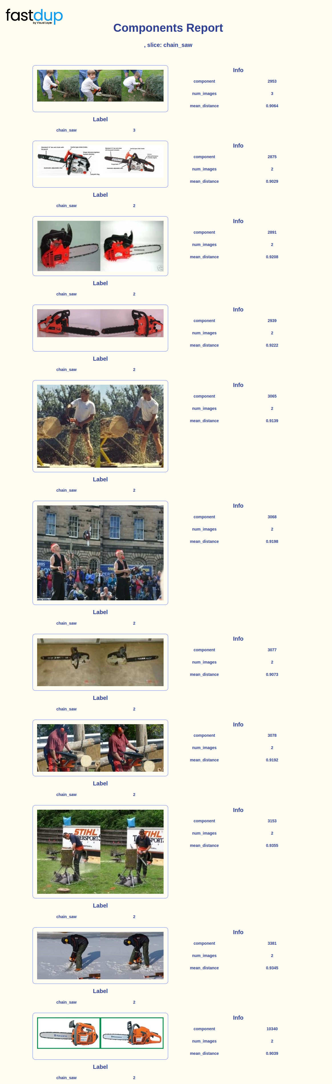

Summary

👍

We now added several important label-specific features to run on top of the raw dataset

Building over the image dataset analysis conducted without labels in the Cleaning and preparing a dataset tutorial, we've seen how to further slice the data and visualize specific classes of interest.

GitHub • Join Slack Community • Discussion Forum Blog • Documentation • About Us LinkedIn • Twitter